NYQUIST Diagram:
Is the open loop Polar plot of the system. From this plot and how it goes around the -1 point on the Polar plot we can tell if the system is stable or not and what the gain and phase margins of the system are.
In the Nyquist plot we calculate the Gain and Phase of the open loop transfer function of the system as the frequency w (rads/s) is varied.
The gain and phase are calculated by substituting jw for s in the Laplace transfer function of the system. Then calculating the magnitude and phase contribution of each term in the derived expression. If the resultant plot encloses the -1 + 0j point then the system will be unstable if the loop is closed.
Example:
Let G(s) = 2 (1 + 2s) / s( 1 + 0.3s)
Let s = jw
G(jw) = 2 (1 + 2jw)/ jw( 1 + 0.3jw)
Gain G(jw) = |G(jw)|
|G(jw)| = 2*Sqrt(1 + (2w)2)/ w*Sqrt(1 + (0.3w)2)
Phase F(jw) = S(Numerator Phase Contributions) - S(Denominator Phase Contributions)
F(jw) = Tan-1(2w/1) - (Tan-1(w/1) + Tan-1(0.3w/1))
We create a table of values as we calculate Gain G(jw) and Phase G(jw) as w is varied. These are then plotted on a Polar plot.
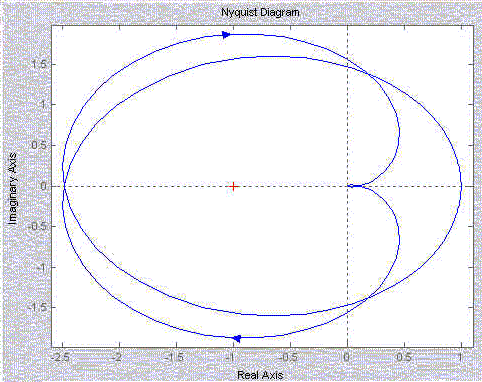
In the most basic case if the resulting plot passes to the left of the -1 point on the real axis and encloses it, the closed loop system will be unstable. The Nyquist diagram below is for an unstable system as it encloses the -1 + 0j point.
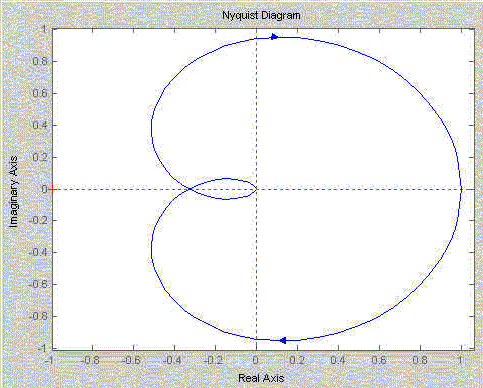
Nyquist diagram for a stable system: -1 + 0j point is not encircled
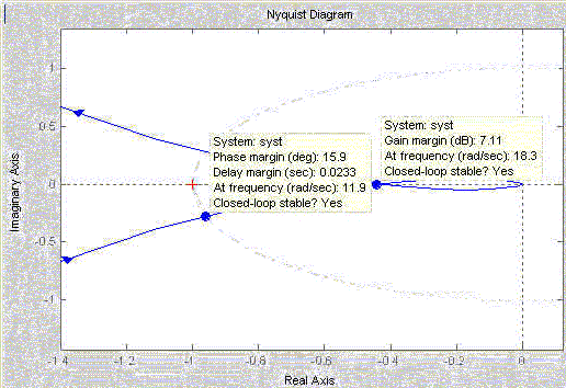
Nyquist diagram for an unstable system: -1 + 0j point is encircled
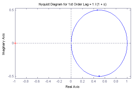
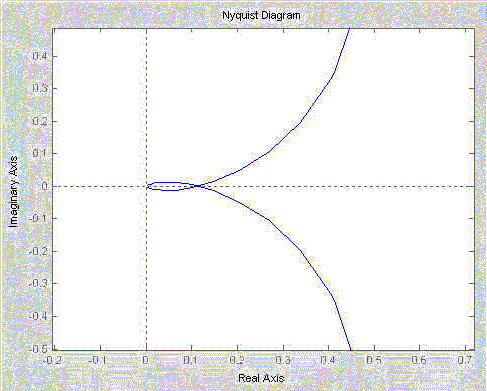
Nyquist plot for a first order system we can neglect the upper part of the plot
why?:
Nyquist plot for second order system of form 1/ (a*s2 + b*s + c):
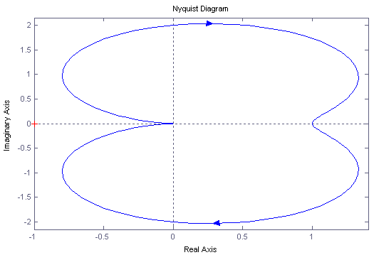
Nyquist plot for third order system of form 1/ (a*s3+ b*s2 + c*s + d):
Nyquist plot for 5th order system of form 1/ (a*s5+ b*s4 +c*s3+ d*s2 + e*s + f)::
Zoomed view of the above plot near the origin:
What can you deduce about the Nyquist plot as the order of the denominator is increased?